Google App Engine

   Google App Engine is a platform for developing and hosting web applications.App engine applications are easy to build, easy to maintain. You can build your application using Python, Java or Go environments. You just upload your application, and it's ready to serve to your users. With App Engine you write your application code, test it on your local machine and upload it to Google. You can create an account and publish an application that people can use right away at no charge from Google, and with no obligation. 

     This tutorial describes how to develop and deploy a simple Python 2.7 project with Google App Engine.  You can build web applications using the Python programming language,  and take advantage of the many libraries, tools and frameworks for Python.A Python web app interacts with the App Engine web server using the WSGI protocol, so apps can use any WSGI-compatible web application framework. App Engine includes a simple web application framework. Apps can use the App Engine Datastore for reliable, scalable persistent storage of data.Apps use the URL Fetch service to access resources over the web, and to communicate with other hosts using the HTTP and HTTPS protocols.
     For our App Engine implementation use Python 2.7v and use the python Software Development Kit(SDK).Download SDK for linux and extract it on your Home folder.You develop and upload Python applications for Google App Engine using the App Engine Python software development kit (SDK).

Let's begin by a simple 'Hello World!' application that show the message 'Hello World! in our browser.

STEP-1
 Create  a directory helloworld. all files for this application reside in this directory. create a file named helloworld.py

CQ40-Notebook-PC:~$ mkdir helloworld
CQ40-Notebook-PC:~$ cd helloworld/
CQ40-Notebook-PC:~/helloworld$ vi helloworld.py

Give the following content in it.

import webapp2

class MainPage(webapp2.RequestHandler):
  def get(self):
      self.response.headers['Content-Type'] = 'text/plain'
      self.response.write('Hello, webapp2 World!')

app = webapp2.WSGIApplication([('/', MainPage)],
                              debug=True)

This Python script responds to a request with an HTTP header that describes the content and the display Hello, world!. webapp2 is light weighted web frame work. This webapp2  has two parts a request handler and a WSGIApplication instants that route incoming request to handle based on URLs.

Pygame: Sierpinski triangle

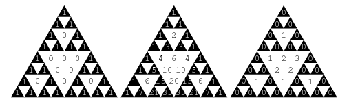
    The Sierpinski triangle is a fractal described by Sierpiński in 1915 and appearing in Italian art from the 13th century. It is also called the Sierpiński gasket. The Sierpinski triangle is a  geometric pattern formed by connecting the  midpoints of the sides of a triangle. It is at the is most  interesting one and   simplest one in fractals.

The Sierpinski triangle is given by Pascal's triangle (mod 2), giving the sequence 1; 1, 1; 1, 0, 1; 1, 1, 1, 1; 1, 0, 0, 0, 1; ... . In other words, coloring all odd numbers black and even numbers white in Pascal's triangle produces a Sierpiński triangle

Construction
An algorithm for obtaining arbitrarily close approximations to the Sierpinski triangle is as follows:

Pygame: Koch Snowflake

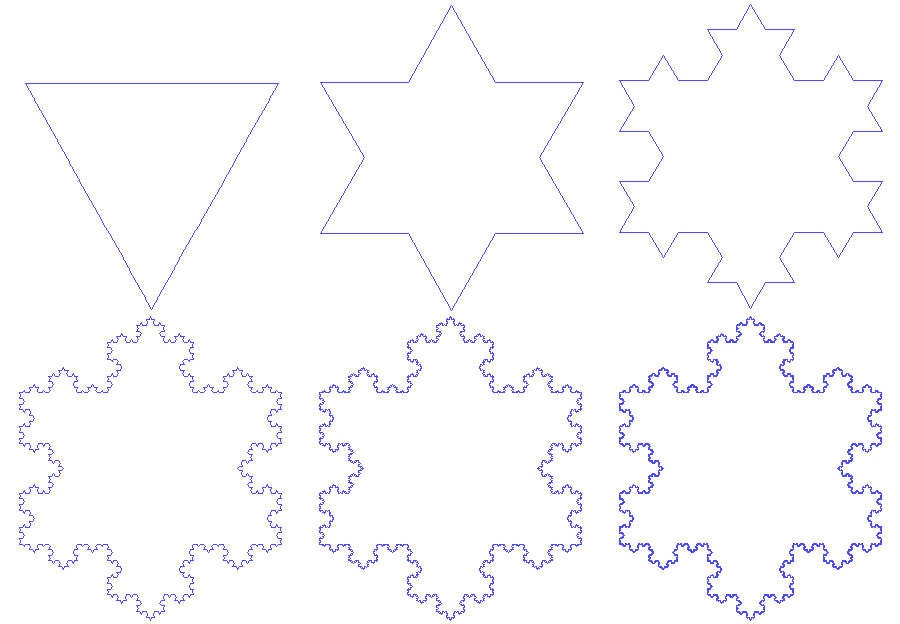
     A factral, also known as the Koch island, which was first described by Helge von Koch in 1904. It is built by starting with an equilateral triangle, removing the inner third of each side, building another equilateral triangle at the location where the side was removed, and then repeating the process indefinitely.

The Koch snowflake (also known as the Koch star and Koch island) is a mathematical curve and one of the earliest fractal curves to have been described.

Construction

The Koch snow flake can be constructed by starting with an equilateral triangle, then recursively altering each line segment as follows:

1. divide the line segment into three segments of equal length.

2. draw an equilateral triangle that has the middle segment from step 1 as its base and points outward.

3.remove the line segment that is the base of the triangle from step 2.

After one iteration of this process, the resulting shape is the outline of a hexagram.

The Koch snowflake is the limit approached as the above steps are followed over and over again. The Koch curve originally described by Koch is constructed with only one of the three sides of the original triangle. In other words, three Koch curves make a Koch snowflake.

   Start with an equilateral triangle T. Scale T by a factor of 1/3 and place 3 copies along each of the three sides of T as illustrated in the diagram below to form a new image S(1). Next scale T by a factor of 1/9 = (1/3)^2 and place 12=4*3 copies along the sides of T(1) as illustrated to form the image S(2). For the next iteration, take 48=4*12 copies of Tscaled by a factor of 1/27=(1/3)^3 and place them around the sides of S(2) to form the image S(3). Continue this construction. The Koch Snowflake is the limiting image of the construction.

Pygame: Game Of Life

Pygame:

    Pygame is a cross-platform set of Python modules designed for writing video games. It includes computer graphics and sound libraries designed to be used with the Python programming language. It is built over the Simple DirectMedia Layer (SDL) library. This is based on the assumption that the most expensive functions inside games (mainly the graphics part) can be abstracted from the game logic, making it possible to use a high-level programming language, such as Python, to structure the game.
    Pygame was originally written by Pete Shinners and is released under the open source free software GNU Lesser General Public License.

Game of life:

    The "game" is a zero-player game, meaning that its evolution is determined by its initial state, requiring no further input. One interacts with the Game of Life by creating an initial configuration and obseving how it evolves.

Rules:

    The universe of the Game of Life is an infinite two-dimensional orthogonal grid of square cells, each of which is in one of two possible states, alive or dead. Every cell interacts with its eight neighbours, which are the cells that are horizontally, vertically, or diagonally adjacent. At each step in time, the following transitions occur:

1. Any live cell with fewer than two live neighbours dies, as if caused by under-population.
2. Any live cell with two or three live neighbours lives on to the next generation.
3. Any live cell with more than three live neighbours dies, as if by overcrowding.
4. Any dead cell with exactly three live neighbours becomes a live cell, as if by reproduction.

The initial pattern constitutes the seed of the system. The first generation is created by applying the above rules simultaneously to every cell in the seed—births and deaths occur simultaneously, and the discrete moment at which this happens is sometimes called a tick (in other words, each generation is a pure function of the preceding one). The rules continue to be applied repeatedly to create further generations.

         I find the best way to understand the Pygame library is to jump straight into an example. In the early days of Pygame, I created The "Conway's game of life". Let's take a look at the code of Conway's game of life. This tutorial will go through the code block by block. Explaining how the code works.

Import modules:

This is the code that imports all the needed modules into your program. It also checks for the availability of some of the optional pygame modules.

import pygame,sys
from pygame.locals import *

Part4: Debugging in R

  Debugging tools are built with R do not part of any package. There are couple of indications that something is not right. It could be a diagnostic message something to happed.Basically three type of main indications.

1. message: A generic notification/diagnostic message produced by the message function; execution of the function continues 
2. warning: An indication that something is wrong but not necessarily fatal;execution of the function continues generated by the warning function 
3. error: An indication that a fatal problem has occurred; execution stops;produced by the stop function

condition: A generic concept for indicating that something unexpected can occur; programmers can create their own conditions

So this is our basic warning,  take a log of negative number

>log(-1)
[1] NaN
Warning message:
In log(-1) : NaNs produced

Part3: Reading and Writing Data in R

Reading Data    Large data objects will usually be read as values from external files rather than entered during an R session at the keyboard. R input facilities are simple and their requirements are fairly strict and even rather inflexible. If variables are to be held mainly in data frames, as we strongly suggest they should be, an entire data frame can be read directly with the read.table() function. There is also a more primitive input function, scan(), that can be called directly. There are a few principal functions reading data into R.  read.table, read.csv, for reading tabular data The read.table function is one of the most commonly used functions for reading data. It has a few important arguments: file, the name of a file, or a connection header, logical indicating if the file has a header line sep, a string indicating how the columns are separated colClasses, a character vector indicating the class of each column in the dataset nrows, the number of rows in the dataset comment.char, a character string indicating the comment character skip, the number of lines to skip from the beginning stringsAsFactors, should character variables be coded as factors For small to moderately sized datasets, you can usually call read.table without specifying any other arguments data <- read.table("foo.txt") R will automatically skip lines that begin with a # and figure out how many rows there are (and how much memory needs to be allocated). Figure what type of variable is in each column of the table. Telling R all these things directly makes R run faster and more efficiently. read.csv is identical to read.table except that the default separator is a comma.

Part2: R-Language Basics

 Data Types and Basic Operations:

1. Objects:
   In every computer language variables provide a means of accessing the data stored in memory. R does not provide direct access to the computer’s memory but rather provides a number of specialized data structures we will refer to as objects.These objects are referred to through symbols or variables.

R has five basic or atomic classes of objects:

1. characters
2. numeric(real numbers)
3. integer
4. complex
5. logical(True or False)

2. Basic types:

2.1 Vectors:

The most basic object in R is vector. A vector can only contain objects of the same class. But the exception is a 'list', which is represent  as a vector but can contain objects of different classes. Empty vectors can be created with the vector() function.

 2.2 Lists:
Lists are another kind of data storage. Lists have elements, each of which can contain any type of R object, i.e. the elements of a list do not have to be of the same type.